The problems with multilayer perceptrons

One of the problems with multilayer perceptrons (MLPs) in the previous post is that they do not take advantage of existing spatial/temporal structures in the data. The other is because every node in a layer is connected to every other node in the next layer the number of parameters that must be learned quickly becomes unwieldy to perform optimization in usefull time. New architectures of neural networks like convolutional neural networks have been very successfull by tackling these two problems.

Convolutional neural networks

To tackle the first issue, activations in layers are allowed to have multiple dimensions. This includes the input layer where the data is feed to the network preserving its existing dimensions (1D for a signal, 2D for images, 3D videos, etc)

To tackle the second issue, activations in a layer are only dependant of a subset of activations in the previous layer and parameters are shared with all other activations. Each set of parameters is called filter, kernel or feature detector and learn to detect relationships of local activations that might appear anywhere. Because of these two properties the number of parameters that need to be learned is greatly reduced.

Although it might seem like this neural network would miss non-local relationships within the data, as we go in deeper layers of the neural network we see more complex relationships emerge from simpler ones.

“Convolution”

The word convolution in these networks comes from the fact that activations of a layer are convolved with these filters to generate the activations for the next layer. Bellow is an animation of how this works in practice.

In the edges of the input layer there isn’t enough data to perform a convolution operation. We can either skip these activations (which will change the size of the layer) or specify a padding \(p\) to fill up data so it is possible to perform a convolution with the edge at the center (and keep the same dimensionality in the “output” layer). Stride \(s\) is how big a jump the convolution operator takes between convolutions. Which in the example above was 1. \(f\) is the size of the filter that is being convolved with the input.

To calculate the size of a curent layer in a given dimension \(n\) based on the size of previous layer \(n^{l-1}\), \(s\) \(p\) and \(f\) we do the operation bellow.

\[n=\frac{n^{l-1}+2*p-f}{s}+1\]

Example convolution neural network (LeNet-5)

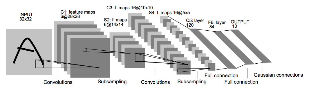
Above is an example of a Convolutional Neural Network known as Lenet-5.

Far left is the input data which consists of a 32 by 32 pixel grey image. Followed by that is layer C1 which will have the result of the convolutions of 6 different filters. The filters size, padding and strides will be such that the activations of this layer will be 28 by 28. Layer S2 will perform what is called max pooling, this is not a convolution operation but instead merely reduces the size of the previous layer by picking the maximum value within areas (or volumes) of the previous layer. The goal with this is to gain some invariance to where an activated feature is located. Layers C3 and S4 are a repetition of C1 and S2 and C5 F6 and Output layers are similar to the MLP approach having flattened S4 to a 1D input.

Let’s implement this in Tensorflow.

First we define methods that will create the diferent types of layers.

def CreateConvLayer(previousLayer, filterCount, filterSize):
    return tf.layers.conv2d(previousLayer, filterCount, filterSize, padding="valid", activation=tf.nn.relu)

def CreatePoolingLayer(previousLayer, pool_size):
    return tf.layers.max_pooling2d(previousLayer, pool_size, pool_size)

def CreateFCNLayer(previousLayer, num_outputs, activation=tf.nn.relu):
    return tf.layers.dense(previousLayer, num_outputs, activation=activation)

We also define a helper function that will give us the size of the filter we need to use to go from a layer with a given size to the layer size we want.

def CalculateFilterSizeFromOutput(inputSize, outputSize, padding=0, stride=1):
    return -((outputSize-1)*stride-inputSize-2*padding)

We then create the computation graph in Tensorflow terminology and the cost function to optimize

X = tf.placeholder(tf.float32, shape=(None, 28, 28, 1))
y = tf.placeholder(tf.float32, shape=(None, 10))

l0 = tf.pad(X, [[0, 0], [2, 2], [2, 2], [0, 0]])
l1 = CreateConvLayer(l0, 6, CalculateFilterSizeFromOutput(32, 28))
l2 = CreatePoolingLayer(l1, 2)
l3 = CreateConvLayer(l2, 16, CalculateFilterSizeFromOutput(14, 10))
l4 = CreatePoolingLayer(l3, 2)
l5 = tf.layers.Flatten()(l4)
l6 = CreateFCNLayer(l5, 120)
l7 = tf.layers.dropout(l6, 0.4)
l8 = CreateFCNLayer(l7, 84)
l9 = tf.layers.dropout(l8, 0.4)
l10 = CreateFCNLayer(l9, 10, None)
cost = tf.reduce_mean(tf.nn.softmax_cross_entropy_with_logits_v2(logits=l10, labels=y))
optimizer = tf.train.AdamOptimizer(learning_rate=0.01).minimize(cost)

To notice l7 and l9 are dropout layers. This is simply a technique to avoid overfitting in which connections are randomly not used to make sure that the predictions cannot rely to much on any given relationship and are forced to generalize the final output.

A remark to pay attention is that although the number of parameters in these networks decreases relative to MLPs the number of hyperparameters and architecture decisions increases. Trying multiple architectures becomes a necessity.

We then run the optimizer to update the parameters of the network so the loss function is minimized like bellow. We use the MNIST data set in this example.

with tf.Session() as sess:
    sess.run([tf.global_variables_initializer(), tf.local_variables_initializer()])
    mnist = input_data.read_data_sets("MNIST_data/", one_hot=True)
    for step in range(20000):
        train = mnist.train.next_batch(100)
        X_train = train[0].reshape(-1, 28, 28, 1)
        y_train = train[1]
        _, c, acc = sess.run([optimizer, cost, accuracy], feed_dict={X: X_train, y: y_train})

        test = mnist.test.next_batch(50)
        X_test = test[0].reshape(-1, 28, 28, 1)
        y_test = test[1]
        acc2 = sess.run([accuracy], feed_dict={X: X_test, y: y_test})
        if step % 2000:
            print("[Step %s] Cost: %s Accuracy (Train): %s Accuracy (Test): %s" % (step, c, acc[0], acc2[0]))

After some time this network should approach 99% accuracy in classifying grey images of handwritten digits. Download the full code here.

This post was about creating a neural network that takes advantage of the convolutional operator but ultimately ends up with a traditional multi layer perceptron for the output.

In the next post I’ll discuss why you would want to do without the fully connected approach in the last layers and build a network that contains convolutions from beginning to end.

Implementing a Convolutional Neural Network

The problems with multilayer perceptrons

Convolutional neural networks

“Convolution”

Example convolution neural network (LeNet-5)

Next