TensorFlow Basics (2/2): Neural Networks
As I wrote in the previous post, TensorFlow is then an engine to apply optimization on arbitrary computation graphs. This task is at the core of most machine learning algorithms where we find the parameters for a that combined with existing data produce good predictions. The objective is to then apply the learned function and parameters to new data to predict outcomes.
Classification on linear structure
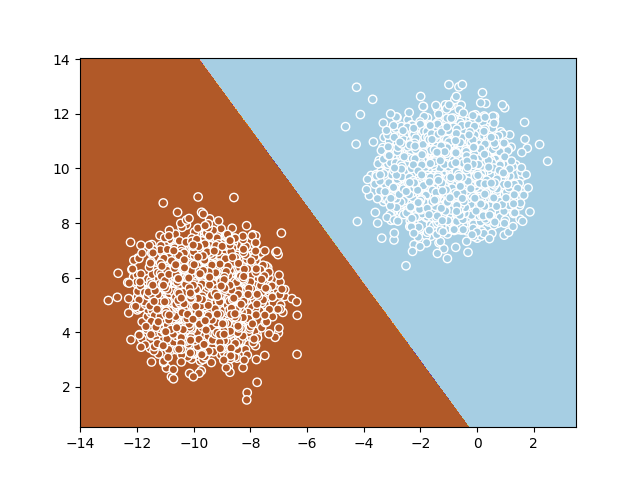
Let’s first use TensorFlow to find a decision boundary on a dataset that is linearly separable.
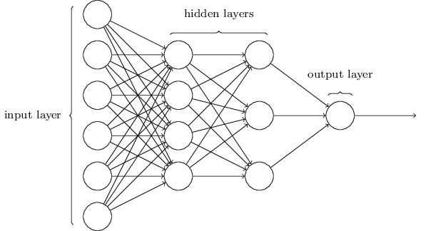
We will use a Perceptron to do this. In short the perceptron function outputs a number between 0 and 1 based on a linear combination of the inputs of the function like illustrated bellow.

|
|
|
Defining this in tensorflow goes like:
Wn = 2
X = tf.placeholder(tf.float32, shape=(None, Wn))
y = tf.placeholder(tf.float32, shape=(None, 1))
W = tf.Variable(tf.random_normal([1, Wn]), dtype=tf.float32)
b = tf.Variable(tf.zeros([1, 1]), dtype=tf.float32)
z = tf.add(tf.matmul(X, tf.transpose(W)), b)
a = 1 / (1 + tf.exp(-z))
cost = tf.losses.log_loss(y, a)
\(X\) and \(y\) are like tensorflow constants but we define them as placeholders because we will only have them later (this will be the data).
\(z\) is the function that performs a linear combination of \(X\) and adds a bias \(b\) and function \(a\) turns the output of \(z\) into a number between 0 and 1.
\(W\) and \(b\) are the paramaters we would like to learn to minimize the \(cost\) of predicting things wrong.
Lets create some linearly separable data feed it to the computation graph and run the optimization that minimizes the loss function. This will find the variables that combined with the data produces the best possible predictions.
X_data, y_data = make_blobs(n_samples=5000, centers=2, n_features=Wn)
m = X_data.shape[0]
optimizer = tf.train.GradientDescentOptimizer(0.01).minimize(cost)
init = tf.global_variables_initializer()
with tf.Session() as sess:
    sess.run(init)
    for epoch in range(1000):
        sess.run(optimizer, feed_dict={X: X_data, y: y_data.reshape(m, 1)})
Once we have found the parameters that minimize the cost function for the given data we can pass new data to make new predictions like:
y_newdata = sess.run(a, feed_dict={X: X_newdata}) > 0.5Bellow is an illustration of the decision boudary that the perceptron learns. Full source code here.
|
|
|
Classification on non-linear structure
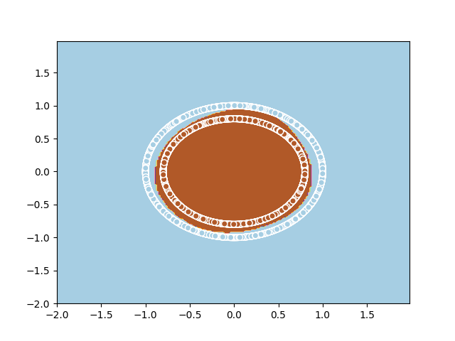
Let’s now use TensorFlow to find a decision boundary on a dataset that is NOT linearly separable.
Building on the previous example I will build a multi layer perceptron neural network. While before we had a vector with the weights of the perceptron now we will have a matrix with weights of multiple perceptrons. Also the output of the perceptrons will feed to other perceptrons in layers with the final layer outputing a number between 0 and 1. This combination of multi layered perceptrons allows for the network as a whole to learn non-linear decision boundaries.
|
|
|
def CreateLayer(previousLayer, perceptronCount):
    _, n = previousLayer.get_shape().as_list()
    W = tf.Variable(tf.random_normal([perceptronCount, n]), dtype=tf.float32)
    b = tf.Variable(tf.zeros([1, perceptronCount]), dtype=tf.float32)
    z = tf.add(tf.matmul(previousLayer, tf.transpose(W)), b)
    a = 1 / (1 + tf.exp(-z))
    return a

Wn = 2
X = tf.placeholder(tf.float32, shape=(None, Wn))
y = tf.placeholder(tf.float32, shape=(None, 1))
l1 = CreateLayer(X, 50)
l2 = CreateLayer(l1, 50)
l3 = CreateLayer(l2, 1)
cost = tf.losses.log_loss(y, l3)
Lets create some non linearly separable data feed it to the computation graph and run the optimization that minimizes the loss function. This will find the variables that combined with the data produces the best possible predictions.
_data, y_data = make_circles(n_samples=5000)
m = X_data.shape[0]
optimizer = tf.train.GradientDescentOptimizer(0.01).minimize(cost)
init = tf.global_variables_initializer()
with tf.Session() as sess:
    sess.run(init)
    for epoch in range(5000):
        sess.run(optimizer, feed_dict={X: X_data, y: y_data.reshape(m, 1)})
Bellow is an illustration of the decision boudary that the perceptron learns. Full source code here.
|
|
|
Next
Next up we will create diferent architectures then the one in the multilayer perceptron to decrease complexity and take advantage of existing structure in the data.