Implementing a neural algorithm of artistic style
In this post we will implement in Tensorflow, as close as possible, the work done by Gatys et al which creates novel representations of existing images in the style of paintings.
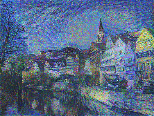
Bellow an example created by this implementation.
|
|
|
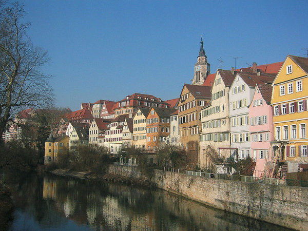
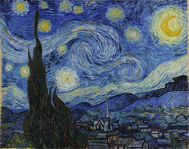
This as been created by combining the images bellow containing content and style.
|
|
|
|
|
All the code excerpts here were taken from the complete source code.
For full disclaimer you can probably find much faster implementations and extensions to the original work.
Motivation
The motivations for this implementation and article are:
- Show (myself) the flexibility of Tensorflow by using pre-trained networks to create novel things.
- Show (myself) how good CNNs are at learning fine and coarse grained representations of spatial data.
Methodology
In a previous post I trained a convolutional neural network (CNN) to identify digits. That network can be seen as a very complex (non-linear) function that, given an image, outputs which digit is in that image.
How good these predictions are is measured by a new function that depends on the networks output and training consists of finding the right parameters of the network that bring us to good predictions.
In neural algorithm for artistic style we start with a VGG19 network pre-trained to detect categories on the imagenet dataset dataset and what we want to learn is the “input” (which we will refer as generated image) that gives us the best combination between the content and style images.
This combination of content and style is based on the activations this generated input creates in this pre-trained network as it flows through it. So let’s take a moment to have an intuition on what these activations represent.
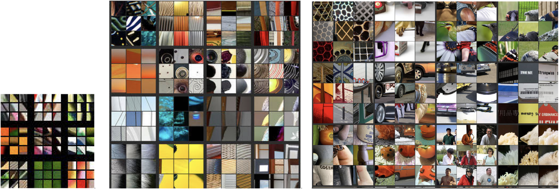
Bellow are images taken from a paper that helps to understand CNNs and shows which images generate the higher activations at different channels in different layers of a network trained in the imagenet dataset.
|
|
|
To make a long story short, the insight is that earlier layers (at the leftmost side) recognize very simple concepts like edges and as you go in deeper layers (to the right) the network learns more and more abstract concepts like eyes in the layer 2 and people in layer 3.
This is important to understand how neural artistic style captures the concepts of content and style.
The intuition to this algorithm is that it specifies content as activations at a certain layer so that if our content image contains a house and a dog, those elements should also be in the generated picture. It also specifies style as how often activations at specific layers co-occur often, so if the style of painting is dominated by brush strokes of blue and white, round yellow circles and houses with dark roofs they should also appear somewhere in the final generated image.
A maybe shorter and easier intuition is that the algorithm will try to make sure high abstract concepts of the content image are present in the generated image and to bring them there will also force bringing activations that co-occur often in the style of the painting.
We encapsulate these ideas into a loss function that will be dependent on the generated, content and style images but we optimize it only with respect to the generated image and apply an optimization algorithm like we have been doing in past posts.
Content
So part of the network will generate a new image that will have the same content as an image that I will call from now on content image.
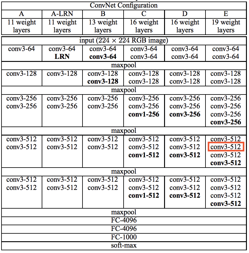
As I wrote above we can define the content of an image as the encoding of the activations at a specific layer in the network. Earlier activations in the network will represent simpler concepts like borders between colors and later activations will represent abstract concepts like trees, houses, clouds etc. We want to pick a layer that combines the right amount of detail and abstract concepts. I will follow the original paper and choose the 2nd convolution in the 4th block of the VGG19 (the 10th layer, marked in red in the image bellow).
|
|
|
We want our generated image activations in this layer to be as close as possible to the activations in the same layer for our content image (remember only our generated image will change and our content will not so we calculate only once the activations for the content image and store them as a constant in our graph to optimize.) This is represented by \(P_{ij}^l\) where \(l\) is the 10th layer and \(i\) and \(j\) are the spatial dimensions of activations at \(l\).
The activations of the generated image will need to be calculated every step of back-propagation and are represented by \(F_{ij}^l\).
Having these two matrices we define the loss function bellow (taken from original paper)
\[L_{content}(\vec{p},\vec{x},l) =\frac{1}{2}\sum_{i,j}(F_{ij}^l - P_{ij}^l)^2\]To implement this in Tensorflow we use the L2 loss function like bellow.
def ContentLoss(F, P):
    return tf.nn.l2_loss(F - P)
Style
Defining style will be based on the same concept as defining the content but with two differences.
- We will use activations of multiple layers
- We will not use the activations directly but the correlation between activations within the same layer which we will refer to as Gram Matrix.
So if at a layer \(l\) we have 256 channels detecting 256 concepts our gram matrix will contain \(256*256\) numbers representing how often each concept happens with every other concept.
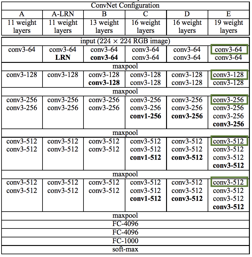
Following the original paper I’ve used layers 1, 3, 5, 9 and 13 (basically all the convolutional layers followed by the pooling layer). See bellow for reference.
|
|
|
Bellow is the formula from the original paper to calculate the Gram Matrix at level \(l\).
\[G_{ij}^l = \sum_{k}F_{ik}^l F_{jk}^l\]Looks more complicated then it is since it boils down to multiplying the activation matrix by itself. We do that in python like bellow.
def GramMatrix(layer):
    _, h, w, c = layer.get_shape().as_list()
    F = tf.reshape(layer, [h*w, c])
    return tf.matmul(tf.transpose(F), F)
We do this for both the style image \(A_{ij}^l\) and the generated image \(G_{ij}^l\) (again we only need to calculate the gram matrix for the style image once since only the generated image will change during training).
We then want that the style for the content and style image to be as close as possible and we define that as bellow (taken from the original paper). In a nutshell it is the average difference of the gram matrices.
\[E_{l} =\frac{1}{4N_{l}^2M_{l}^2}\sum_{i,j}(G_{ij}^l - A_{ij}^l)^2\]Implementation in Tensorflow bellow.
def StyleLoss(A, G, M, N):
    return tf.nn.l2_loss(G - A) / (2*N**2*M**2)
Finally, because we want to apply style in multiple layers, we define style loss as the average style difference at multiple layers. Like defined bellow.
\[L_{style}(\vec{a},\vec{x}) = \sum_{l=0}^Lw_{l}E_{l}\]...
styleLoss = reduce(tf.add,
[StyleLoss(A[l],
G[l],
M[l],
N[l]) for l in STYLE_LAYERS])
styleLoss /= len(STYLE_LAYERS)
...Loss function
We then plug in both style and content loss functions together with two empirically found hyperparameters \(\alpha\) and \(\beta\) to arrive at the total loss function we want to minimize with Tensorflow. and defined bellow.
\[L(\vec{p},\vec{a},\vec{x}) = \alpha L_{content}(\vec{p},\vec{x}) + \beta L_{style}(\vec{a},\vec{x})\]alpha = 10e-5
beta = 5
loss = alpha * contentLoss + beta * styleLossThis was the only detail which i departed from the original paper because I found these hyperperameters gave a more pleasing combination of content and style.
Pre-trained network
So like I wrote above we:
we start with a VGG19 network pre-trained to detect categories on the imagenet dataset dataset
I’ve used the VGG19 Keras application to extract the weights of every layer in the network like bellow.
def getWeights():
    with tf.Graph().as_default():
        weights = VGG19(weights='imagenet', include_top=False).get_weights()
    return weights
I then wrote a function to create the part of the VGG19 network I was interested in working with. Notice that I used average pooling instead of max pooling like described in the original paper.
def getActivations(X, weights, debug=False):
    layers = [2, 2, 4, 4, 1]
    activations = {}
    w = 0
    for i in range(len(layers)):
        for j in range(layers[i]):
            with tf.name_scope("block{}_{}".format(i+1, j+1)):
                conv_W = tf.constant(weights[w], name="W")
                conv_b = tf.constant(weights[w+1], name="b")
                conv = tf.nn.conv2d(X,
                                    conv_W,
                                    strides=[1, 1, 1, 1],
                                    padding='SAME') + conv_b
                relu = tf.nn.relu(conv)
                activations["relu{}_{}".format(i+1, j+1)] = relu
                if debug:
                    tf.summary.histogram("weights", conv_W)
                    tf.summary.histogram("bias", conv_b)
                    tf.summary.histogram("relu", relu)
                X = relu
                w += 2
        if i+1 is not 5:
            with tf.name_scope("pool{}".format(i+1)):
                X = tf.nn.pool(X, [2, 2], "AVG", "VALID", strides=[2, 2])
    return activations
Training
This should look familiar. Point out I’m explicitly telling the optimizer which variable can be updated.
optimizer = tf.train.AdamOptimizer(5).minimize(loss, var_list=[x])

config = tf.ConfigProto(device_count={'GPU': 1}, log_device_placement=True)
with tf.Session(config=config) as sess:
    writer = tf.summary.FileWriter("logs", sess.graph)
    tf.summary.scalar("loss", loss)
    tf.summary.image("preview", x[..., ::-1], max_outputs=1)
    summaryOp = tf.summary.merge_all()
    sess.run(tf.global_variables_initializer())

    for epoch in range(5000):
        _, summary = sess.run([optimizer, summaryOp])
        writer.add_summary(summary, epoch)
Results
So optimizing this network when using the two images bellow as content and style.
|
|
|
|
|
|
We arrive at the generated image bellow.
|
|
|
|
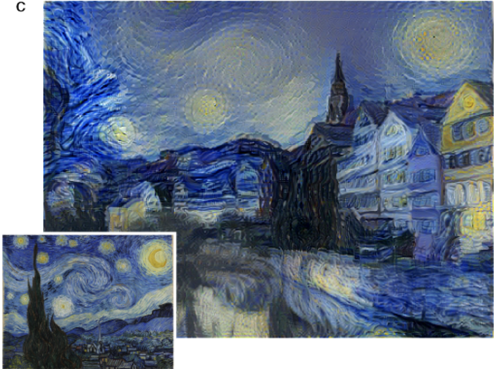
I’ve purposefully picked these two images to see if I would arrive at the same result as the original paper.
|
|
|
|
|
|
Putting the two side by side it seems the example in the original paper is much more smooth. But I was pleased enough with the approximation to call it implemented.
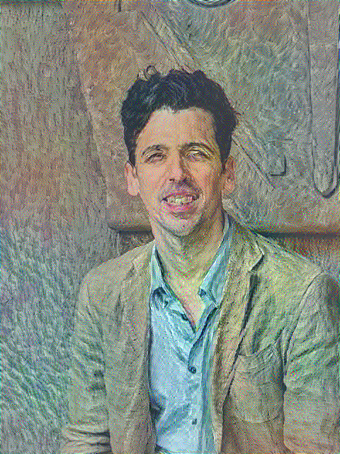
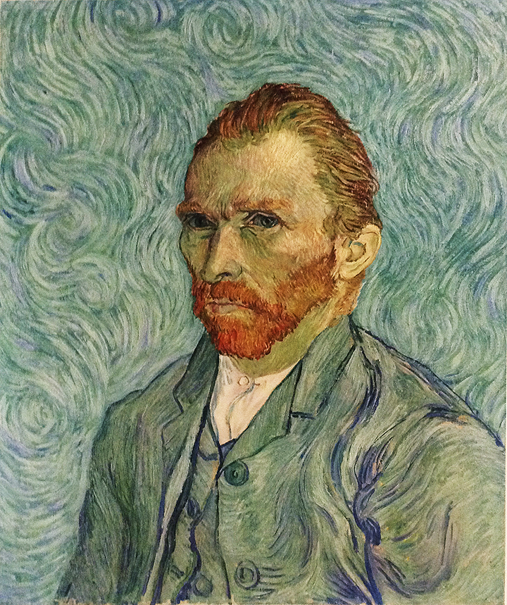
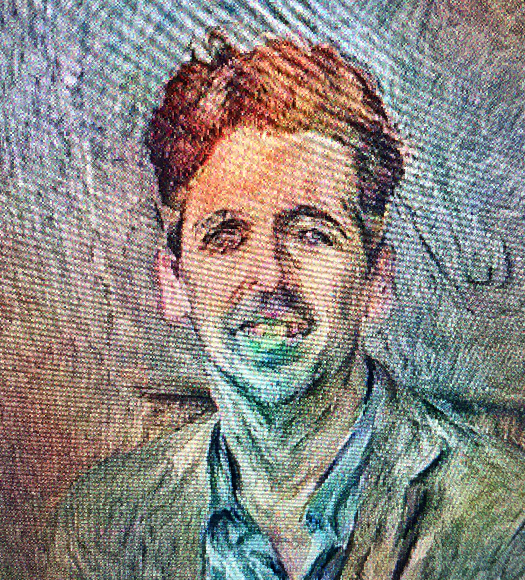
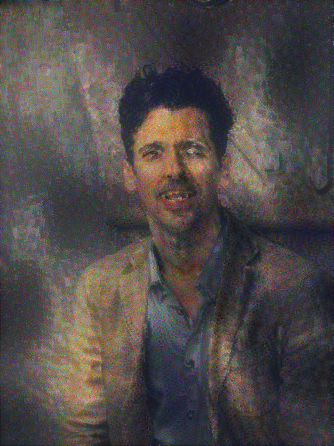
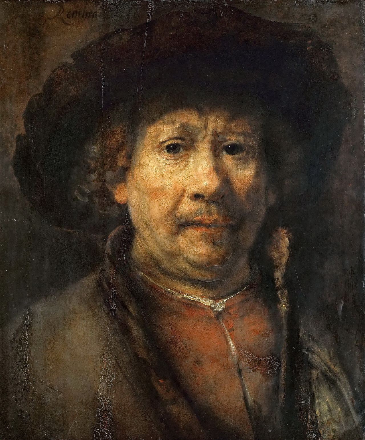
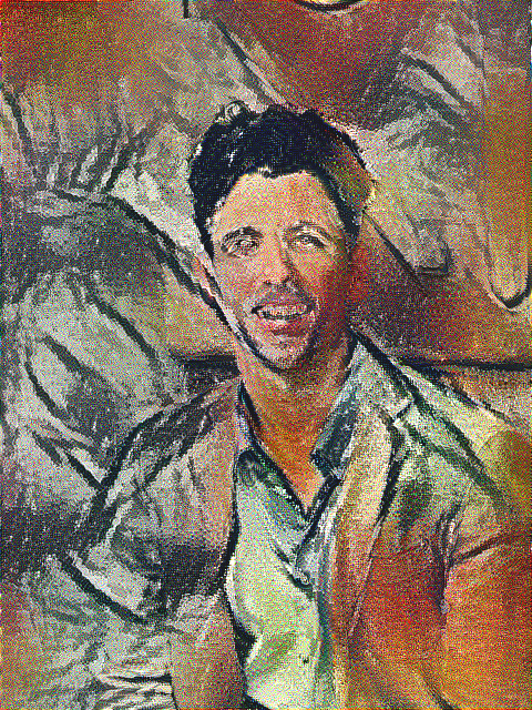
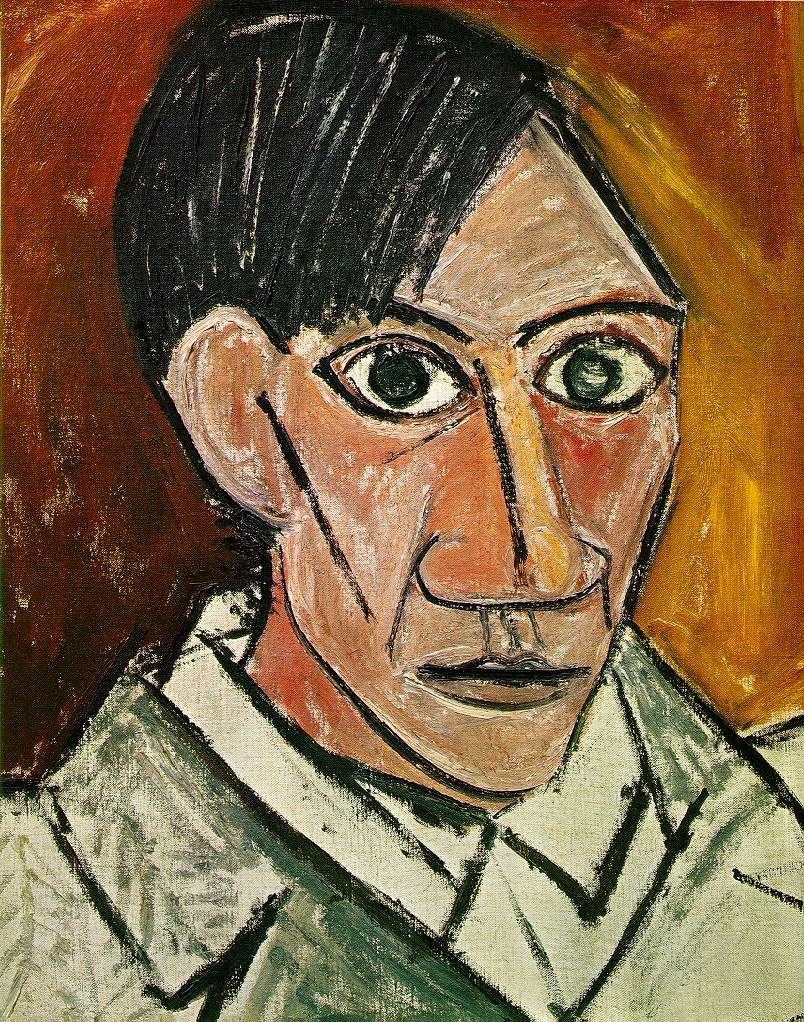
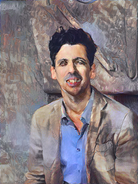
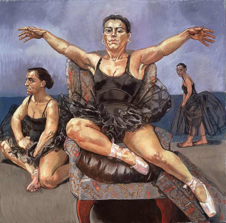
I’ve also tried to create a self-portrait for fun with styles I like (see bellow).
|
|
|
|
|
Interestingly enough when I was trying different \(\alpha\) and \(\beta\) values and increased the weight of the style considerably the generated image produced my hair in the same color as Van Goghs.
|
|
|
|
|
|
|
|
|
|
|
|
|
|
|
|
|
|
All the code excerpts here were taken from the complete source code.